The first step in using any spreadsheet is getting some data! This tutorial will show you different ways to import some of your portfolio data into a spreadsheet and how to format it to make it easier to read.
Getting Data
The first step to using any spreadsheet is getting some data – once we have our data in our sheet, we will then start formatting it to make it easier to use.
Copy/Paste Method
The easiest way to import data is to just copy and paste it from a website or another source.
Getting Your Historical Portfolio Values
To get your old portfolio values, you can copy and paste them out of the HTMW website. First, you will need to get your historical portfolio values from the HTMW website. You can find these on the “Graph My Portfolio” page.
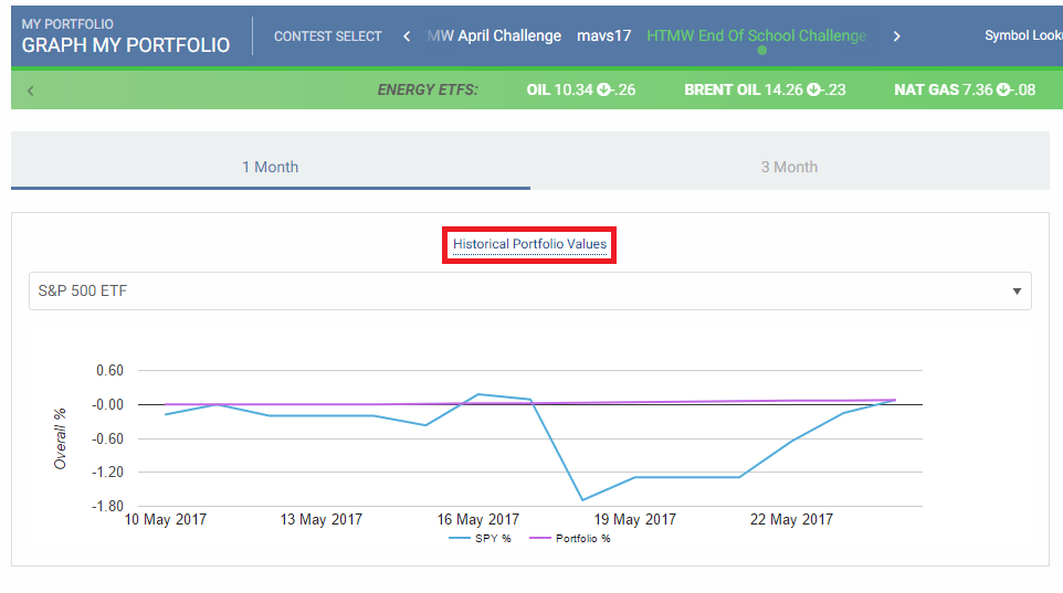
This will open up a small window showing what your portfolio value was for every day of the contest. Highlight the information you want, then right click and “Copy”.
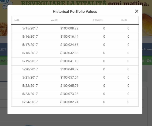
Next, open a new blank spreadsheet and click cell A1. You can then right-click and “Paste” the data in. The column headings should be included too.
Adding Column Headings
If the column headings are not included, right-click the first row and select “Insert Row”. This will add a new row to the top of the spreadsheet where you can type in the column names. Google sheets gives you the option to add a row above or below the one you right clicked.

Now “Save” your file somewhere you can easily find it later, you’ve got some data!
Getting Historical Prices for Stocks
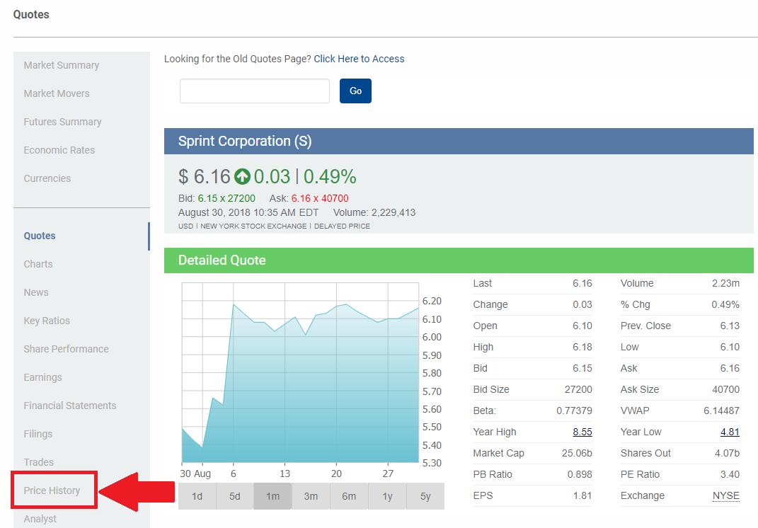
For this example, we want to get the historical prices for a stock, so we can look at how the price has been moving over time. First, create a new blank spreadsheet in Excel or Google Sheets. We will use Sprint stock (symbol: S). Go to the quotes page and search for S, then click “Price History” on the right side of the page:
Next, change the “Start” and “End” dates to the time you want to look at. For this example, we will use the same dates that we saved for our portfolio values, January 11 through January 15, 2016. Once you load the historical prices, highlight everything from “Date” to the last number under “Adj. Close” (it should look like this):
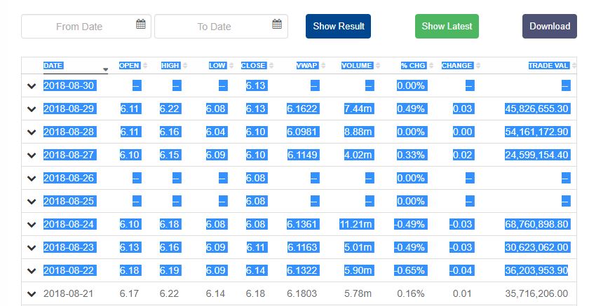
Now copy the data, select cell A1 in your blank spreadsheet, and paste.
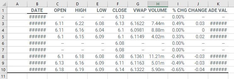
Congratulations, we have now imported some data into our spreadsheet! You can now save it for future use. The data is a bit messy; we will look at formatting later.
Export Method
Sometimes, websites will make it easy for you to export data directly to your spreadsheet without copy/paste. If an export option is available, this is going to work better, since it will require less formatting later.
If we look back at the Historical Prices, you can see that there is also a “Download” button at the top of the table:
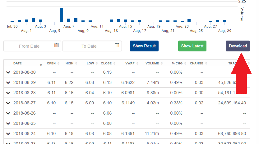
This will download a spreadsheet you can just open directly – you can also see the data is already easier to read and better formatted, which will save us time later.
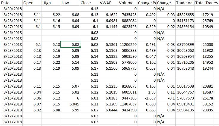
Copying Between Spreadsheets
You can also export your portfolio data from the My Contests page – this will download one big spreadsheet showing your account balances, trades, open positions, and more:

Once you download the spreadsheet, you can open it to see the available data:
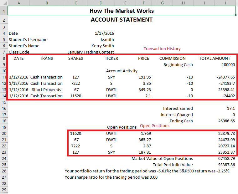
The top red square is your transaction history, the bottom red square is your Open Positions. To use this data, you will need to open a new blank spreadsheet and copy these boxes (just like we did above) from one spreadsheet to another.
Start by taking your “Transaction History”, copying the data, and pasting it into a new spreadsheet.
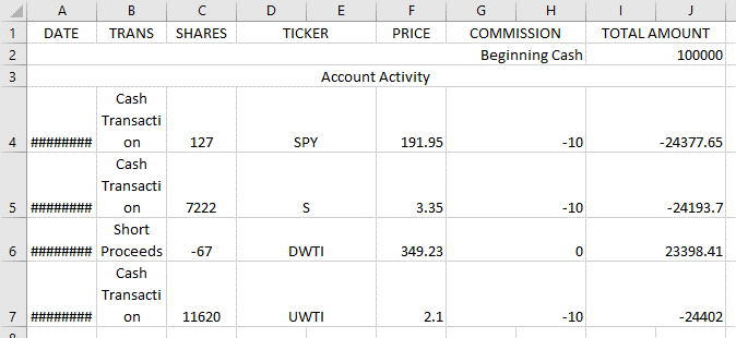
To start using this data, we will need to look at formatting to make it easier to read.
Formatting Your Data
Now that we have a few saved spreadsheets, we can look at formatting the data to make it easy to read and use later.
Changing Data Order
If we look at the spreadsheets we have saved for our Historical Portfolio Values, it is the exact opposite of what we have for our Historical Prices.
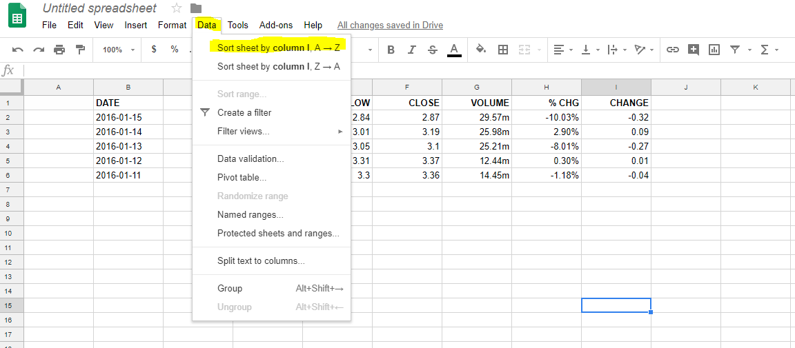
To get them in the same order, we will want to open up our Historical Prices spreadsheet, and order the data from “Oldest” to “Newest”.
We will use the “Sort” function with Excel, or the “Data” function for Google Sheets.
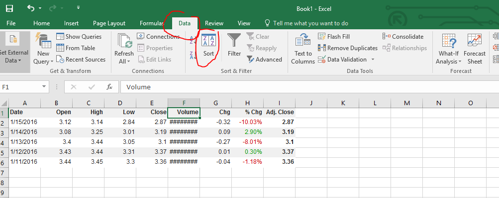
We can now choose what we want to sort by, and how to sort it. If you click the drop-down menu under “Sort By”, excel lists all the column headings it detects (select “Date “). Next, under “Order”, we want “Oldest to Newest “:
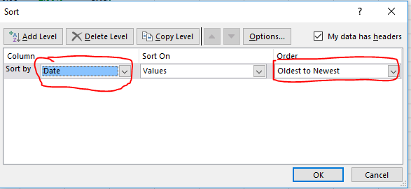
Now your data should be in the same order as your portfolio values from earlier.
Changing Column Width
Next, you’ll notice that some of your data appears just as “########”. This is not because there is an error, the number is just too big to fit in the width of our cell. To fix this, we can increase and decrease the widths of our cells by dragging the boundaries between the rows and columns:

Tip: if you double click these borders, the cell to the left will automatically adjust its width to fit the data in it.
If you want to automatically adjust all your cells at once, at the top menu click “Format”, and “Auto Fit Column Width”:
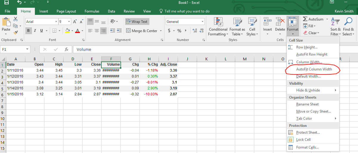
Once you’ve adjusted your volume column, everything should be visible!
Removing Columns
If we want to use this data for making a graph, we will not need all of the data in the sheet. We really only need the “Date” and “Closing Price”. To keep it easy to read, we will delete some of the extra data.
If you just highlight the data you don’t need and press “Delete”, you will end up with a bunch of blank cells, which is not very useful when trying to read the table:

Instead, click on “B” and drag all the way to “H” to select the full columns:

Now right-click and click “Delete”, and the entire rows will disappear. Now the Close will be your new column B, with no more empty space. You now have your historical price data, so save this excel file so you can use it later.
Unmerging Cells
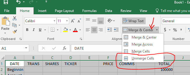
Now let’s go back to our Transaction History spreadsheet. With this sheet, we cannot do many of the basic operations because there are some “Merged Cells”. Merged Cells can be used for formatting and presentation, but for now it is just getting in our way.
This is the case with the Ticker, Commission, and Total Amount cells. We need to “unmerge” these cells to make our data usable.

To do this, select all your data, then on the main menu bar click on “Merge and Center “. Under this, click “Unmerge Cells”. On Google Sheets, this can be done by clicking on the “Format” tab in the navigation bar and then clicking on “Text Wrapping” and then “Clip”.
Putting It All Together
Now that we have our data all in their own cells, we can start deleting the rows and columns we don’t need. For example, rows 2 and 3 have our beginning cash, which we don’t need in our transaction history. Columns E and H are now blank, so we can get rid of those too. Once you delete the rows and columns you don’t need, you can also autofit the row width to make the “date” visible.


 Effective Tools for Businesses to Protect Sensitive Data
 How Interest Rates Affect Bond Prices